planet.donarmstrong.com

Previously in this series:

• The “lost boarding pass” puzzle
• The “deadly board game” puzzle
• The “knight on an infinite chessboard” puzzle
• The “largest stock profit or loss” puzzle
• The “birthday paradox” puzzle
• The “Spelling Bee honeycomb” puzzle
• Feller’s “coin-tossing” puzzle

I love 538’s Riddler column, and the April 10 puzzle is another interesting one. I’ll quote:

Over the course of three days, suppose the probability of any spammer making a new comment on this week’s Riddler column over a very short time interval is proportional to the length of that time interval. (For those in the know, I’m saying that spammers follow a Poisson process.) On average, the column gets one brand-new comment of spam per day that is not a reply to any previous comments. Each spam comment or reply also gets its own spam reply at an average rate of one per day.

For example, after three days, I might have four comments that were not replies to any previous comments, and each of them might have a few replies (and their replies might have replies, which might have further replies, etc.).

After the three days are up, how many total spam posts (comments plus replies) can I expect to have?

This is a great opportunity for tidy simulation in R, and also for reviewing some of the concepts of stochastic processes (this is known as a Yule process). As we’ll see, it’s even thematically relevant to current headlines, since it involves exponential growth.

Solving a puzzle generally involves a few false starts. So I recorded this screencast showing how I originally approached the problem. It shows not only how to approach the simulation, but how to use those results to come up with an exact answer.

Simulating a Poisson process

The Riddler puzzle describes a Poisson process, which is one of the most important stochastic processes. A Poisson process models the intuitive concept of “an event is equally likely to happen at any moment.” It’s named because the number of events occurring in a time interval of length \(x\) is distributed according to \(\mbox{Pois}(\lambda x)\), for some rate parameter \(\lambda\) (for this puzzle, the rate is described as one per day, \(\lambda=1\)).

How can we simulate a Poisson process? This is an important connection between distributions. The waiting time for the next event in a Poisson process has an exponential distribution, which can be simulated with rexp().

# The rate parameter, 1, is the expected events per day
waiting <- rexp(10, 1)
waiting

##  [1] 0.1417638 2.7956808 1.2725448 0.3452203 0.5303130 0.2647746 2.6195738
##  [8] 1.2933250 0.5539181 0.9835380

For example, in this case we waited 0.14 days for the first comment, then 2.8 after that for the second one, and so on. On average, we’ll be waiting one day for each new comment, but it could be a lot longer or shorter.

You can take the cumulative sum of these waiting periods to come up with the event times (new comments) in the Poisson process.

qplot(cumsum(waiting), 0)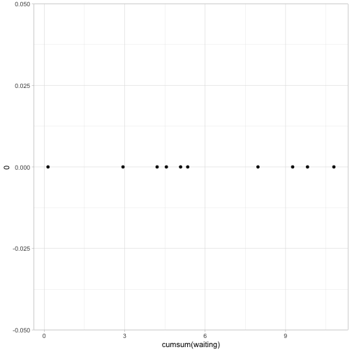

Simulating a Yule process

Before the first comment happened, the rate of new comments/replies was 1 per day. But as soon as the first comment happened, the rate increased: the comment could spawn its own replies, so the rate went up to 2 per day. Once there were two comments, the rate goes up to 3 per day, and so on.

This is a particular case of a stochastic process known as a Yule process (which is a special case of a birth process. We could prove a lot of mathematical properties of that process, but let’s focus on simulating it.

The waiting time for the first commentwould be \(\mbox{Exponential}(1)\), but the waiting time for the second is \(\mbox{Exponential}(2)\), then \(\mbox{Exponential}(3)\), and so on. We can use the vectorized rexp() function to simulate those. The waiting times will, on average, get shorter and shorter as there are more comments that can spawn replies.

set.seed(2020)

waiting_times <- rexp(20, 1:20)

# Cumulative time
cumsum(waiting_times)

##  [1] 0.2938057 0.9288308 1.0078320 1.1927956 1.4766987 1.6876352 2.5258522
##  [8] 2.5559037 2.6146623 2.6634295 2.7227323 2.8380710 2.9404016 2.9460719
## [15] 2.9713356 3.0186731 3.1340060 3.2631936 3.2967087 3.3024576

# Number before the third day
sum(cumsum(waiting_times) < 3)

## [1] 15

In this case, the first 15 events happened before the third day. Notice that in this simulation, we’re not keeping track of which comment received a reply: we’re treating all the comments as interchangeable. This lets our simulation run a lot faster since we just have to generate the waiting times.

All combined, we could perform this simulation in one line:

sum(cumsum(rexp(20, 1:20)) < 3)

## [1] 6

So in one line with replicate(), here’s one million simulations. We simulate 300 waiting periods from each, and see how many happen before the first day.

sim <- replicate(1e6, sum(cumsum(rexp(300, 1:300)) < 3))

mean(sim)

## [1] 19.10532

It looks like it’s about 19.1.

Turning this into an exact solution

Why 19.1? Could we get an exact answer that is intuitively satisfying?

One trick to get a foothold is to vary one of our inputs: rather than looking at 3 days, let’s look at the expected comments after time \(t\). That’s easier if we expand this into a tidy simulation, using one of my favorite functions crossing().

library(tidyverse)
set.seed(2020)

sim_waiting <- crossing(trial = 1:25000,
         observation = 1:300) %>%
  mutate(waiting = rexp(n(), observation)) %>%
  group_by(trial) %>%
  mutate(cumulative = cumsum(waiting)) %>%
  ungroup()

sim_waiting

## # A tibble: 7,500,000 x 4
##    trial observation waiting cumulative
##    <int>       <int>   <dbl>      <dbl>
##  1     1           1  0.294       0.294
##  2     1           2  0.635       0.929
##  3     1           3  0.0790      1.01 
##  4     1           4  0.185       1.19 
##  5     1           5  0.284       1.48 
##  6     1           6  0.211       1.69 
##  7     1           7  0.838       2.53 
##  8     1           8  0.0301      2.56 
##  9     1           9  0.0588      2.61 
## 10     1          10  0.0488      2.66 
## # … with 7,499,990 more rows

We can confirm that the average number of comments in the first three days is about 19.

sim_waiting %>%
  group_by(trial) %>%
  summarize(num_comments = sum(cumulative <= 3)) %>%
  summarize(average = mean(num_comments))

## # A tibble: 1 x 1
##   average
##     <dbl>
## 1    18.9

But we can also use crossing() (again) to look at the expected number of cumulative comments as we vary \(t\).

average_over_time <- sim_waiting %>%
  crossing(time = seq(0, 3, .25)) %>%
  group_by(time, trial) %>%
  summarize(num_comments = sum(cumulative < time)) %>%
  summarize(average = mean(num_comments))

(Notice how often “solve the problem for one value” can be turned into “solve the problem for many values” with one use of crossing(): one of my favorite tricks).

How does the average number of comments increase over time?

ggplot(average_over_time, aes(time, average)) +
  geom_line()

At a glance, this looks like an exponential curve. With a little experimentation, and noticing that the curve starts at \((0, 0)\), we can find that the expected number of comments at time \(t\) follows \(e^t-1\). This fits with our simulation: \(e^3 - 1\) is 19.0855.

ggplot(average_over_time, aes(time, average)) +
  geom_line(aes(y = exp(time) - 1), color = "red") +
  geom_point() +
  labs(y = "Average # of comments",
       title = "How many comments over time?",
       subtitle = "Points show simulation, red line shows exp(time) - 1.")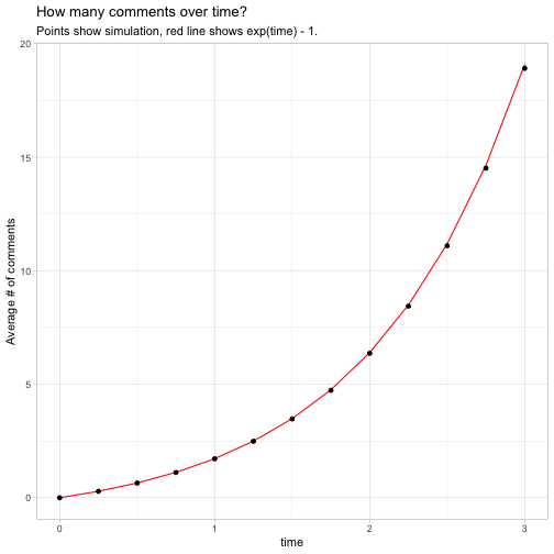

Intuitively, it makes sense that on average the growth is exponential. If we’d described the process as “bacteria in a dish, each of which could divide at any moment”, we’d expect exponential growth. The “minus one” is because the original post is generating comments just like all the others do, but doesn’t itself count as a comment.¹

Distribution of comments at a given time

It’s worth noting we’re still only describing an average path. There could easily be more, or fewer, spam comments by the third day. Our tidy simulation gives us a way to plot many such paths.

sim_waiting %>%
  filter(trial <= 50, cumulative <= 3) %>%
  ggplot(aes(cumulative, observation)) +
  geom_line(aes(group = trial), alpha = .25) +
  geom_line(aes(y = exp(cumulative) - 1), color = "red", size = 1) +
  labs(x = "Time",
       y = "# of comments",
       title = "50 possible paths of comments over time",
       subtitle = "Red line shows e^t - 1")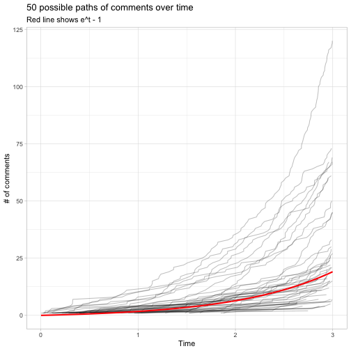

The red line shows the overall average, reaching about 19.1 at 3 days. However, we can see that it can sometimes be much smaller or much larger (even even more than 100).

What is the probability distribution of comments after three days- the probability there is one comment, or two, or three? Let’s take a look at the distribution.

# We'll use the million simulated values from earlier
num_comments <- tibble(num_comments = sim)

num_comments %>%
  ggplot(aes(num_comments)) +
  geom_histogram(binwidth = 1)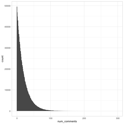

Interestingly, at a glance this looks a lot like an exponential curve. Since it’s a discrete distribution (with values 0, 1, 2…), this suggests it’s a geometric distribution: the expected number of “tails” flipped before we see the first “heads”.

We can confirm that by comparing it to the probability mass function, \((1-p)^np\). If it is a geometric distribution, then because we know the expected value is \(e^3-1\) we know the rate parameter \(p\) (the probability of a success on each heads) is \(\frac{1}{e^3}=e^{-3}\).

p <- exp(-3)

num_comments %>%
  filter(num_comments <= 150) %>%
  ggplot(aes(num_comments)) +
  geom_histogram(aes(y = ..density..), binwidth = 1) +
  geom_line(aes(y = (1 - p) ^ num_comments * p), color = "red")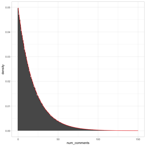

This isn’t a mathematical proof, but it’s very compelling. So what we’ve learned overall is:

\(X(t)\sim \mbox{Geometric}(e^{-t})\) \(E[X(t)]= e^{-t}-1\)

These are true because the rate of comments is one per day. If the rate of new comments were \(\lambda\), you’d replace \(t\) above with \(\lambda t\).

I don’t have an immediate intuition for why the distribution is geometric. Though it’s interesting that the parameter \(p=e^{-t}\) for the geometric distribution (the probability of a “success” on the coin flip that would stop the process) is equal to the probability that there are no events in time \(t\) for a Poisson process.

Conclusion: Yule process

I wasn’t familiar with it when I first tried out the riddle, but this is known as a Yule process. For confirmation of some of the results above you can check out this paper or the Wikipedia entry, among others.

What I love about simulation is how it builds an intuition for these processes from the ground up. These simulated datasets and visualizations are a better “handle” for me for grasp the concepts than mathematical equations would be. After I’ve gotten a feel for the distributions, I can check my answer by looking through the mathematical literature.