planet.donarmstrong.com

My new office introduced me to a betting game I wasn’t previously familiar with: Super Bowl squares. It’s played with a ten-by-ten grid, like this one from printyourbrackets.com:

Each row and column gets an assortment of digits from 0-9 representing each team’s score, and each person playing the game (after putting in some money) adds their initials to one of the boxes. Then the winner is picked based on the least significant digit of the score. If (for example) the game ended up being Eagles 20-Patriots 24, the player who had picked the row with 0 and the column with 4 would win.

If your team sets the digits in advance, you can get a statistical edge. Since not every score is equally likely, the least-significant digits aren’t equally likely either. Here I’ll take a data-driven approach to find the most common digits, and pairs of digits, in NFL scores. Like in most of my posts, I’ll be using the R language and the tidyverse collection of packages. By the end of tonight you can see how my predictions did!

Most common digits

We could use just the Super Bowl scores, perhaps scraped from Wikipedia. In a perfect world we could use that data, since Super Bowl scores are likely to be subtly different than the regular season. But there’ve been only 51, so the data is rather noisy. Instead, we’ll look at all NFL games since 1978, thanks to this helpful GitHub dataset from James Every.

library(tidyverse)
theme_set(theme_light())

# Git clone first from git@github.com:devstopfix/nfl_results.git
games <- dir("nfl_results/", pattern = ".csv", full.names = TRUE) %>%
  map_df(read_csv)

# Gather into one tall data frame of scores, and calculate the digit
# The dataset has a couple games from before 1978, but only a few per year
scores <- games %>%
  filter(season >= 1978) %>%
  gather(type, score, home_score, visitors_score) %>%
  mutate(digit = score %% 10)

scores

## # A tibble: 18,148 x 8
##    season  week kickoff             home_team  visitin… type   score digit
##     <int> <int> <dttm>              <chr>      <chr>    <chr>  <int> <dbl>
##  1   1978     1 1978-09-02 00:00:00 Buccaneers Giants   home_…    13  3.00
##  2   1978     1 1978-09-03 00:00:00 Bears      Cardina… home_…    17  7.00
##  3   1978     1 1978-09-03 00:00:00 Bengals    Chiefs   home_…    23  3.00
##  4   1978     1 1978-09-03 00:00:00 Bills      Steelers home_…    17  7.00
##  5   1978     1 1978-09-03 00:00:00 Broncos    Raiders  home_…    14  4.00
##  6   1978     1 1978-09-03 00:00:00 Browns     49ers    home_…    24  4.00
##  7   1978     1 1978-09-03 00:00:00 Eagles     Rams     home_…    14  4.00
##  8   1978     1 1978-09-03 00:00:00 Falcons    Oilers   home_…    20  0   
##  9   1978     1 1978-09-03 00:00:00 Jets       Dolphins home_…    33  3.00
## 10   1978     1 1978-09-03 00:00:00 Lions      Packers  home_…     7  7.00
## # ... with 18,138 more rows

This gives us a set of over 18,000 football scores (from over 9,000 games) we can analyze.

First we could ask what the most common scores are. (If you’re a football fan, you may want to try guessing before you look at them!)

scores %>%
  count(score, sort = TRUE)

## # A tibble: 60 x 2
##    score     n
##    <int> <int>
##  1    17  1412
##  2    20  1197
##  3    24  1189
##  4    10  1089
##  5    13   952
##  6    14   946
##  7    27   931
##  8    21   810
##  9    31   781
## 10    23   754
## # ... with 50 more rows

The most commmon (by a wide margin) is 17. This could come from two touchdowns (each with an extra point, or one with two extra points) and a field goal. 27 is also common, so 7 as the least significant digit is already looking like a solid bet.

So let’s create a histogram of the most common final digits. (I’ll do this one in silver for the Eagles).

ggplot(scores, aes(digit)) +
  geom_histogram(fill = "#8D9093", binwidth = .5) +
  scale_x_continuous(breaks = 0:9) +
  labs(title = "Frequency of final digits in NFL games since 1966")

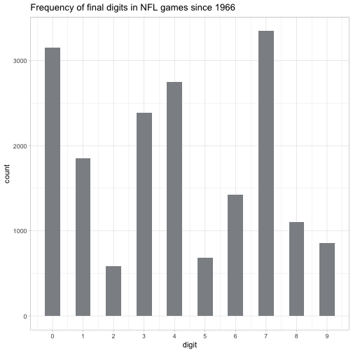
As we suspected, the most common digit is 7. It’s closely followed by 0, and 4 and 5 are pretty common as well. But you really don’t want to bet on 2 or 5.

Are they independent?

It’s likely that each team’s strategy influences the other (and both may be influenced by common factors such as the weather or referee), meaning that the two digits in a score aren’t statistically independent. So let’s consider the most common pairs of scores. For this graph we’ll use red and white for the Patriots.

games %>%
  count(home_digit = home_score %% 10,
        visitors_digit = visitors_score %% 10) %>%
  mutate(percent = n / sum(n)) %>%
  ggplot(aes(home_digit, visitors_digit, fill = percent)) +
  geom_tile() +
  scale_x_continuous(breaks = 0:9) +
  scale_y_continuous(breaks = 0:9) +
  scale_fill_gradient2(high = "#C8102E", low = "white",
                       labels = scales::percent_format()) +
  theme_minimal() +
  labs(x = "Last digit of home team score",
       y = "Last digit of visitor team score",
       title = "Common pairs of NFL scores",
       fill = "% of games since 1978")

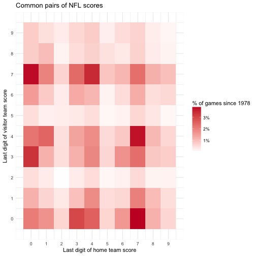
(Super Bowl games don’t actually have a home and away team, but it’s a reasonable way to visualize this data).

Interestingly, even though 7 and 0 are themselves the most common digits, the most common pairs of digits are not pairs of 7s or pairs of zeroes, but rather 7-0 and 0-7. This makes sense because except in rare circumstances, games are almost never tied, since they would go into overtime. This means that while 17 and 20 are both common scores, 17-17 and 20-20 are very rare (in fact, in this dataset there are only two of each).

Change over time

Rules and strategies change over time, and it’s plausible that the ending digits have changed with it. We can examine this hypothesis with a line graph.

scores %>%
  count(decade = 10 * season %/% 10,
        digit) %>%
  mutate(digit = reorder(digit, -n)) %>%
  group_by(decade) %>%
  mutate(percent = n / sum(n)) %>%
  ggplot(aes(decade, percent, color = digit)) +
  geom_line() +
  scale_y_continuous(labels = scales::percent_format()) +
  expand_limits(y = 0) +
  labs(title = "Most common ending digits of NFL games by decade",
       y = "% of scores ending in this digit")

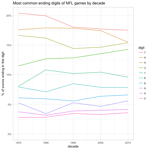
Not too much: the relative ordering of the 10 digits has stayed the exact same across each decade. It looks like 7 has become a little less common, and that 0 and 4 have mostly converged in frequency.

We could consider filtering for only a subset of the data, such as games since 1990. If we consider too many years, it won’t be a precisely accurate picture of modern football, but if we consider too few we won’t have enough data and the estimate will be noisy (This is a classic example of a bias-variance tradeoff). Some sophisticated models can balance the two concerns, but this graph shows it probably isn’t worth the effort.

Conclusion

The pairs I’d bet on are 7-0/0-7 or 4-7/7-4, the most common pairings of digits. (Though the chance of winning with each is still around 3%, not much higher than winning a roulette spin). If those are taken I’d generally avoid pairs of the same digit, since the lack of ties make them unusually uncommon (last year’s Super Bowl game was the first to ever go into overtime, and there has never been a tied score).

In a more sophisticated model we’d consider rates within each team, and possibly incorporate the Vegas odds (a winning team’s score distribution is different than a losing team). I might try that for Super Bowl LIII next year.

Good luck and enjoy the game!