planet.donarmstrong.com

Like a lot of people, I was intrigued by “I Am Part of the Resistance Inside the Trump Administration”, an anonymous New York Times op-ed written by a “senior official in the Trump administration”. And like many data scientists, I was curious about what role text mining could play.

Ok NLP people, now’s your chance to shine. Just spitballing here but TF-IDF on “the op-ed” compared to the published writing of every senior Trump admin official? I want likelihood estimates with standard errors. GO!

— Drew Conway (@drewconway) September 5, 2018

This is a useful opportunity to demonstrate how to use the tidytext package that Julia Silge and I developed, and in particular to apply three methods:

• Using TF-IDF to find words specific to each document (examined in more detail in Chapter 3 of our book)
• Using widyr to compute pairwise cosine similarity
• How to make similarity interpretable by breaking it down by word

Since my goal is R education more than it is political analysis, I show all the code in the post.

Even in the less than 24 hours since the article was posted, I’m far from the first to run text analysis on it. In particular Mike Kearney has shared a great R analysis on GitHub (which in particular pointed me towards CSPAN’s cabinet Twitter list), and Kanishka Misra has done some exciting work here.

Downloading data

Getting the text of the op-ed is doable with the rvest package.

# setup
library(tidyverse)
library(tidytext)
library(rvest)
theme_set(theme_light())

url <- "https://www.nytimes.com/2018/09/05/opinion/trump-white-house-anonymous-resistance.html"

# tail(-1) removes the first paragraph, which is an editorial header
op_ed <- read_html(url) %>%
  html_nodes(".e2kc3sl0") %>%
  html_text() %>%
  tail(-1) %>%
  data_frame(text = .)

The harder step is getting a set of documents representing “senior officials”. An imperfect but fast approach is to collect text from their Twitter accounts. (If you find an interesting dataset of, say, government FOIA documents, I recommend you try extending this analysis!)

We can look at a combination of two (overlapping) Twitter lists containing administration staff members:

• CSPAN’s list of Cabinet accounts
• digiphile’s list of White House staff

library(rtweet)

cabinet_accounts <- lists_members(owner_user = "CSPAN", slug = "the-cabinet")
staff <- lists_members(slug = "white-house-staff", owner = "digiphile")

# Find unique screen names from either account
accounts <- unique(c(cabinet_accounts$screen_name, staff$screen_name))

# Download ~3200 from each account
tweets <- map_df(accounts, get_timeline, n = 3200)

This results in a set of 136,501 from 69 Twitter handles. There’s certainly no guarantee that the op-ed writer is among these Twitter accounts (or, if they are, that they even write their tweets themselves). But it still serves as an interesting case study of text analysis. How do we find the tweets with the closest use of language?

Tokenizing tweets

First, we need to tokenize the tweets: to turn them from full messages into individual words. We probably want to avoid retweets, and we need to use a custom regular expression for splitting it and remove links (just as I’d done when analyzing Trump’s Twitter account).

# When multiple tweets across accounts are identical (common in government
# accounts), use distinct() to keep only the earliest
reg <- "([^A-Za-z\\d#@']|'(?![A-Za-z\\d#@]))"

tweet_words <- tweets %>%
  filter(!is_retweet) %>%
  arrange(created_at) %>%
  distinct(text, .keep_all = TRUE) %>%
  select(screen_name, status_id, text) %>%
  mutate(text = str_replace_all(text, "https?://t.co/[A-Za-z\\d]+|&amp;", "")) %>%
  unnest_tokens(word, text, token = "regex", pattern = reg) %>%
  filter(str_detect(word, "[a-z]"))

This parses the corpus of tweets into almost 1.5 million words.

Among this population of accounts, and ignoring “stop words” like “the” and “of”, what are the most common words? We can use ggplot2 to visualize this.

tweet_words %>%
  filter(!word %in% stop_words$word) %>%
  count(word, sort = TRUE) %>%
  head(16) %>%
  mutate(word = reorder(word, n)) %>%
  ggplot(aes(word, n)) +
  geom_col() +
  coord_flip() +
  labs(y = "# of uses among staff Twitter accounts")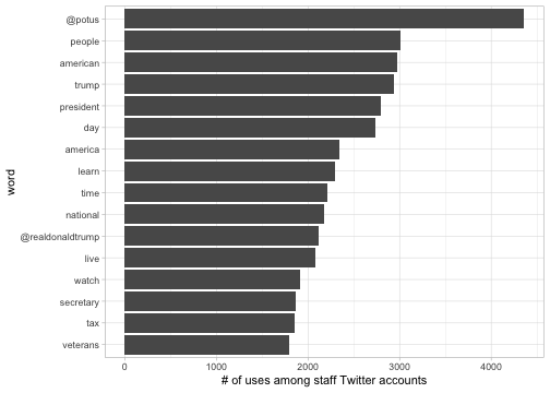

No real surprises here. Many accounts mention @POTUS often, as well as words like “people”, “American”, and “Trump” that you’d expect from administration accounts.

Finding a text signature: TF-IDF vectors

What words make up someone’s “signature”? What make up mine, or Trump’s, or Mike Pence’s, or the op-ed’s?

We could start with the most common words someone uses. But there are some words, like “the” and “of” that just about everyone uses, as well as words like “President” that everyone in our dataset will use. So we also want to downweight words that appear across many documents. A common tool for balancing these two considerations and turning them into a “signature” vector is tf-idf: term-frequency inverse-document-frequency. This takes how frequently someone uses a term, but divides it by (the log of) how many documents mention it. For more details, see Chapter 3 of Text Mining with R.

The bind_tf_idf function from tidytext lets us compute tf-idf on a dataset of word counts like this. Before we do, we bring in the op-ed as an additional document (since we’re interesting in considering it as one “special” document in our corpus).

# Combine in the op_ed wordswith the name "OP-ED" 
op_ed_words <- op_ed %>%
  unnest_tokens(word, text) %>%
  count(word)

word_counts <- tweet_words %>%
  count(screen_name, word, sort = TRUE) %>%
  bind_rows(op_ed_words %>% mutate(screen_name = "OP-ED"))

# Compute TF-IDF using "word" as term and "screen_name" as document
word_tf_idf <- word_counts %>%
  bind_tf_idf(word, screen_name, n) %>%
  arrange(desc(tf_idf))

word_tf_idf

## # A tibble: 226,410 x 6
##    screen_name    word                 n      tf   idf tf_idf
##    <chr>          <chr>            <int>   <dbl> <dbl>  <dbl>
##  1 JoshPaciorek   #gogreen           170 0.0204   4.25 0.0868
##  2 USTradeRep     ustr               147 0.0213   3.56 0.0757
##  3 DeptVetAffairs #vantagepoint      762 0.0173   3.56 0.0614
##  4 DeptofDefense  #knowyourmil       800 0.0185   3.15 0.0584
##  5 DanScavino     #trumptrain        655 0.0201   2.86 0.0575
##  6 USUN           @ambassadorpower   580 0.0154   3.56 0.0548
##  7 USTreasury     lew                690 0.0183   2.86 0.0523
##  8 HUDgov         hud                566 0.0196   2.30 0.0451
##  9 OMBPress       omb                 38 0.0228   1.95 0.0444
## 10 SecElaineChao  'can                 1 0.00990  4.25 0.0421
## # ... with 226,400 more rows

We can now see the words with the strongest associations to a user. For example, Josh Paciorek (the VP’s Deputy Press Secretary) uses the hashtag #gogreen (supporting Michigan State Football) quite often; it makes up 2% of the words (tf, term frequency). Since no one else uses it (leading to an inverse document frequency, idf, of 4.5), this makes it a critical part of his TF-IDF vector (his “signature”).

We could take a look at the “signatures” of a few selected Twitter accounts.

library(drlib)

selected <- c("realDonaldTrump", "mike_pence", "DeptVetAffairs", "KellyannePolls")

word_tf_idf %>%
  filter(screen_name %in% selected) %>%
  group_by(screen_name) %>%
  top_n(12, tf_idf) %>%
  ungroup() %>%
  mutate(word = reorder_within(word, tf_idf, screen_name)) %>%
  ggplot(aes(word, tf_idf, fill = screen_name)) +
  geom_col(show.legend = FALSE) +
  scale_x_reordered() +
  coord_flip() +
  facet_wrap(~ screen_name, scales = "free_y") +
  labs(x = "",
       y = "TF-IDF vectors of this word for this user",
       title = "TF-IDF: top words for selected staff members")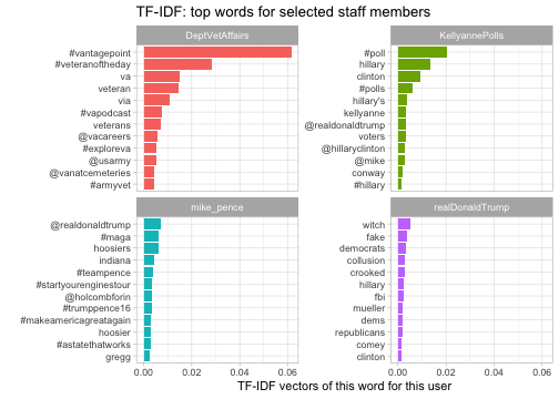

This gives us a set of words that are quite specific to each account. For instance, @DeptVetAffairs uses hashtags like “#vantagepoint” and “#veteranoftheday” that almost no other account in this set would use. Words that are specific to Trump include “witch” (as in “witch hunt”), “fake” (as in “fake news”) and other phrases that he tends to fixate on while other government officials don’t. (See here for my text analysis of Trump’s tweets as of August 2017).

This shows how TF-IDF offers us a vector (an association of each word with a number) that describes the unique signature of that document. To compare our documents (the op-ed with each Twitter account), we’ll be comparing those vectors.

The widyr package: cosine similarity

How can we compare two vectors to get a measure of document similarity? There are many approaches, but perhaps the most common for comparing TF-IDF vectors is cosine similarity. This is a combination of a dot product (multiplying the same term in document X and document Y together) and a normalization (dividing by the magnitudes of the vectors).

My widyr package offers a convenient way to compute pairwise similarities on a tidy dataset:

library(widyr)

# Find similarities between screen names
# upper = FALSE specifies that we don't want both A-B and B-A matches
word_tf_idf %>%
  pairwise_similarity(screen_name, word, tf_idf, upper = FALSE, sort = TRUE)

## # A tibble: 2,415 x 3
##    item1          item2           similarity
##    <chr>          <chr>                <dbl>
##  1 VPComDir       VPPressSec           0.582
##  2 DeptVetAffairs SecShulkin           0.548
##  3 ENERGY         SecretaryPerry       0.472
##  4 HUDgov         SecretaryCarson      0.440
##  5 usedgov        BetsyDeVosED         0.417
##  6 Interior       SecretaryZinke       0.386
##  7 SecPriceMD     SecAzar              0.381
##  8 SecPompeo      StateDept            0.347
##  9 VPPressSec     VP                   0.343
## 10 USDA           SecretarySonny       0.337
## # ... with 2,405 more rows

The top results show that this elementary method is able to match people to their positions. The VP Press Secretary and VP Communications Director unsurprisingly work closely together and tweet on similar topics. Similarly, it matches Shulkin, Perry, Carson, DeVos, and Zinke to their (current or former) cabinet positions, and links the two consecutive Health and Human Services directors (Price and Azar) to each other.

It’s worth seeing this document similarity metric in action, but it’s not what you’re here for. We’re really excited about seeing comparisons between the op-ed and Twitter articles. We can

# Look only at the similarity of the op-ed to other documents
op_ed_similarity <- word_tf_idf %>%
  pairwise_similarity(screen_name, word, tf_idf, sort = TRUE) %>%
  filter(item1 == "OP-ED")

library(drlib)

op_ed_similarity %>%
  head(12) %>%
  mutate(item2 = reorder(item2, similarity)) %>%
  ggplot(aes(item2, similarity)) +
  geom_col() +
  scale_x_reordered() +
  coord_flip() +
  facet_wrap(~ item1, scales = "free_y") +
  labs(x = "",
       y = "Cosine similarity between TF-IDF vectors",
       subtitle = "Based on 69 selected staff accounts",
       title = "Twitter accounts using words similar to NYTimes op-ed")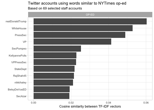

This unveils the most similar writer as… Trump himself.

Hmmm. While that would certainly be a scoop, it doesn’t sound very likely to me. And the other top picks (the official White House account, the Press Secretary, and the Vice President) also seem like suspicious guesses.

Interpreting machine learning: what words contributed to scores?

The method of tf-idf is a fairly basic one for text mining, but as a result it has a useful trait: it’s based on a linear combination of one-score-per-word. This means we can say exactly how much each word contributed to a TF-IDF similarity between the article and a Twitter account. (Other machine learning methods allow interactions between words, which makes them harder to interpret).

We’ll try an approach of decomposing our TF-IDF similarity to see how much each . You could think of this as asking “if the op-ed hadn’t used this word, how much lower would the similarity score be?”

# This takes a little R judo, but it's worth the effort

# First we normalize the TF-IDF vector for each screen name,
# necessary for cosine similarity
tf_idf <- word_tf_idf %>%
  group_by(screen_name) %>%
  mutate(normalized = tf_idf / sqrt(sum(tf_idf ^ 2))) %>%
  ungroup()

# Then we join the op-ed words with the full corpus, and find
# the product of their TF-IDF with it in other documents
word_combinations <- tf_idf %>%
  filter(screen_name == "OP-ED") %>%
  select(-screen_name) %>%
  inner_join(tf_idf, by = "word", suffix = c("_oped", "_twitter")) %>%
  filter(screen_name != "OP-ED") %>%
  mutate(contribution = normalized_oped * normalized_twitter) %>%
  arrange(desc(contribution)) %>%
  select(screen_name, word, tf_idf_oped, tf_idf_twitter, contribution)

# Get the scores from the six most similar
word_combinations %>%
  filter(screen_name %in% head(op_ed_similarity$item2)) %>%
  mutate(screen_name = reorder(screen_name, -contribution, sum),
         word = reorder_within(word, contribution, screen_name)) %>%
  group_by(screen_name) %>%
  top_n(12, contribution) %>%
  ungroup() %>%
  mutate(word = reorder_within(word, contribution, screen_name)) %>%
  ggplot(aes(word, contribution, fill = screen_name)) +
  geom_col(show.legend = FALSE) +
  scale_x_reordered() +
  facet_wrap(~ screen_name, scales = "free_y") +
  coord_flip() +
  labs(x = "",
       y = "Contribution to similarity score",
       title = "What caused each Twitter account to be similar to the article",
       subtitle = "For the 6 accounts with the highest similarity score")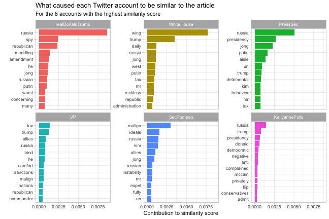

Now the reasons for the TF-IDF similarities become clearer.

The op-ed uses the words “Russia” five times. The Press Secretary and especially Trump mention Russia multiple times on their Twitter accounts, always within the context of defending Trump (as expected). Several accounts also get a high score because they mention the word “Trump” so frequently.

Unfortunately, with a document this short and topical, that’s all it takes to get a high similarity score (a bag of words method can’t understand the context, such as mentioning Russia in a negative or a defensive context). This is one reason it’s worth taking a closer look at what goes into an algorithm,

Having said that, there’s one signature I think is notable.

“Malign behavior”

Many others have noted “lodestar” as a telltale word in the piece. None of the relevant documents included that. I’d like to focus on another word that did: malign. Emphasis mine:

He complained for weeks about senior staff members letting him get boxed into further confrontation with Russia, and he expressed frustration that the United States continued to impose sanctions on the country for its malign behavior.

“Malign” isn’t as rare a word as “lodestar”, but it’s notable for being used in the exact same context (discussing Russia or other countries’ behavior) in a number of tweets from both Secretary of State Pompeo and the @StateDepartment account. (Pompeo has actually used the term “malign” an impressive seven times since May, though all but one were about Iran rather than Russia).

In #Finland tonight. Monday, @POTUS & I will meet with our Russian counterparts in #Helsinki A better relationship with the Russian government would benefit all, but the ball is in Russia’s court. We will continue to hold Russia responsible for its malign activities @StateDept pic.twitter.com/K4C1PSrRMb

— Secretary Pompeo (@SecPompeo) July 15, 2018

“Malign behavior” has been common language for Pompeo this whole year, as it has for other State Department officials like Jon Huntsman. What’s more, you don’t need data science to notice the letter spends three paragraphs on foreign policy (and praises “the rest of the administration” on that front). I’m not a pundit or a political journalist, but I can’t resist speculating a bit. Pompeo is named by the Weekly Standard as one of four likely authors of the op-ed, but even if he’s not the author my guess would be someone in the State Department.

Conclusion: Opening the black box

It’s worth emphasizing again that this article is just my guess based on a single piece of language (it’s nowhere close to the certainty of my analysis of Trump’s Twitter account during the campaign, which was statistically significant enough that I’d be willing to consider it “proof”).

I was fairly skeptical from the start that we could get strong results with document-comparison methods like this, especially on such a small article. That opinion mirrored people with much more expertise than I have:

That means you need a pretty large sample to not have large error bars. Don’t expect conclusive or even suggestive evidence here.

— David Mimno (@dmimno) September 6, 2018

But I’m satisfied with this analysis both as a demonstration of tidytext methods and one on the importance of model interpretability. When we ran a TF-IDF comparison, we knew it was wrong because @realDonaldTrump appeared at the top. But what if Trump hadn’t been the one to mention Russia the most, or if another false positive had caused an account to rise to the top? Breaking similarity scores down by word is a useful way to interrogate our model and understand its output. (See here for a similar article about understanding the components of a model).